Mark Pogson from Quintessa has co-authored a research paper in the journal Medical Engineering & Physics, which uses machine learning to estimate forces exerted on the body while running, based on data from a body-worn sensor.
Biomechanical loads are an important consideration for athletes, but they are difficult to measure outside the laboratory, hence load monitoring tends to focus on physiological metrics such as heart rate, thus giving an incomplete picture of overall training load. Working with collaborators in biomechanics and data science at Liverpool John Moores University, KU Leuven and the University of Birmingham, Mark has developed a machine learning method to estimate biomechanical loads during running activities by using data from an accelerometer attached to the torso, which measures trunk acceleration (TA).
The accelerometer is part of a device which is already widely used by athletes to track their movement using GPS, so the new method provides an easy and cost-effective way to quantify biomechanical loads outside the laboratory by using data which are readily available.
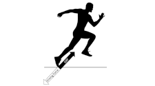
To represent biomechanical load, the method uses the magnitude of ground reaction force (GRF), which is the force exerted on the body when it impacts the ground (Figure 1). GRF can be measured in the laboratory by using a force platform, which allows the relationship with TA, as measured by the accelerometer, to be observed (Figure 2). Although there is a clear association between the two, a mechanical model faces major challenges to predict GRF from the TA signal because the centre of mass of the body continually moves relative to the sensor location.
The method was found to provide excellent estimates of GRF from TA data in many cases, as shown in Figure 3, demonstrating its effectiveness to predict both GRF magnitudes and time dynamics for different athletes and types of impact. Further analysis found that model predictions performed well overall, but some outliers were evident for particularly short and long impacts, which may reflect the distribution of data used for model training.
The method provides promising results which may help athletes to account better for biomechanical loads in their training schedules, thus increasing the effectiveness of training while reducing the risk of injury. With further work, it may be possible to improve GRF estimates by using subject-specific model training and including biophysical data inputs. GRF monitoring is also relevant to healthcare, including for load-dependent conditions such as osteoarthritis, hence similar approaches could be of value in these areas.


